
Author: Ruoyan Han
Code of this project is avaliable at:
https://github.com/Ry2an/case_code/tree/master/bios623as2
Introduction
In 1996, the Australian government exempted a new gun law that banned semiautomatic rifles and pump-action shotguns and started to buyback firearms. Chapman, et al, did an analysis to reveal whether the law change had brought changes in death rates for different reasons related to gunshot [1]. This document is the assignment of BIOS 621 and I will repeat one outcome (total non-firearm death rate) in Chapman, et al’s article with same statistical methods and compare the usage of log negative binomial regression and log Poisson regression in this situation.
Method
Data setting
Rate calculation
Since the total death is gradually growing, comparing the absolute death number change in two law backgrounds could be affected. Therefore, as the same thing the author did, a death rate is calculated by the total death divide by the total person-year at risk for some linear regression calculation in this assignment.
Analysis processes
At the first step, log (mean) and log (standard deviation) of the outcome measure (total non-firearm death) and their stratified results are calculated to see whether the outcome could be recognized as a Poisson distribution. If the outcome is in Poisson distribution, the log(mean) and log (standard deviation) should be similar.
The second step is to calculate the mean and 95% confidence interval of the total non-firearm death rate in two law backgrounds (before 1997 and after 1997). Three solutions are attempt to get the result. The first one is to treat the means of non-firearm death rate before and after the law change are in two sample distributions (t distribution). Therefore, the standard error of the means could be calculated by standard deviation divided by square root of n into two periods of time, where n means that number of means in two periods of time. The degree of freedom is equal to n – 1. The formula is shown as (1).
The second solution of calculating the mean and its 95%confidence interval is by linear regression. The model is shown as (2).
The third solution will use log negative binomial regression to calculate the mean and confidence interval of the total non-firearm death rate before and after the law change. The model is shown as (3). (in Negative Binomial Regression)
By assuming law change is an effect modifier of the relationship between time (year) and total non-firearm death rate, three models shown in the article has been fitted. The formula is shown as (4) – (6). (in Negative Binomial Regression)
A log Poisson regression is also fitted to compare with model The model formula is shown as (7).
Model (6) and model (7) are compared by Akaike information criterion (AIC), log (likelihood of regression), diagnose plots and regression curve with residuals. In order to compare the intercept change at the year of the law update, I will use ‘(year - 1996)’ to replace the original ‘year’ in the model (6) and model (7).
Software:
The software I used for calculation and analysis in this assignment are R software 3.6.1 and MS Office Excel 2019.
R packages and tools used: R markdown; MASS; ggplot2; plotrix; plyr; countreg; gridExtra
Results
The total log mean and log standard deviation for total non-firearm deaths rate is 2.41 and 0.32.
The log mean and log standard deviation before the law change for total non-firearm deaths rate is 2.36 and 0.27.
The log mean and log standard deviation after the law change for total non-firearm deaths rate is 2.46 and 0.17.
Log mean and log standard deviation of outcome is not similar. Therefore, we cannot assume that the log outcome is in a Poisson distribution.
Mean calculation and interpret.
Solution 1 gave us the average rate of total non-firearm death before the law change is 10.61 (95% CI: 8.64, 12.57) deaths per 100000 person-years. The average rate of total non-firearm death before the law change is 11.80 (95% CI: 9.83, 13.76) deaths per 100000 person-years.
Solution 2 gave us the average rate of total non-firearm death before the law change is 10.61 (95% CI: 10.00, 11.21) deaths per 100000 person-years. The average rate of total non-firearm death before the law change is 11.80 (95% CI: 11.19, 12.40) deaths per 100000 person-years.
Solution 1 gave us the average rate of total non-firearm death before the law change is 10.61 (95% CI: 10.09, 11.16) deaths per 100000 person-years. The average rate of total non-firearm death before the law change is 11.79 (95% CI: 11.21, 12.41) deaths per 100000 person-years.
A plot has generated to describe the mean calculation from three solutions.
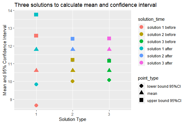
Fig 1. Results of three solutions to calculate mean non-firearm death rate before and after the law change
Table 1. Regression result
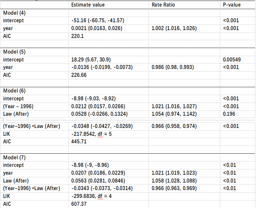
From the result, we can know that in the year of 1979 to 1996 before the law change, the average trend of total non-firearm death rate is 1.002 (rate ratio) from model (4), while in the year of 1997 to 2013 after the law change, the trend of total non-firearm death rate is 0.986 (rate ratio). The change of this difference in log of the rate ratio is -0.0348 (the change of slope of two period log(rate ratio)) from model 6 and this difference is statistically significant.
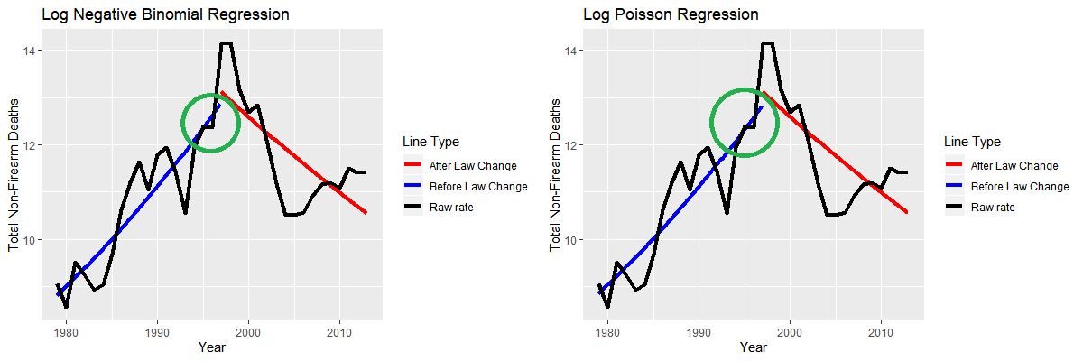
Fig 2. Predicted Values of Model (6) (Left) and Model (7) (Right)
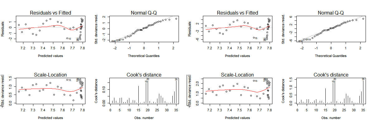
Fig 3. Diagnostic Plots of Model (6) (Left 4 plots) and Model (7) (Right 4 Plots)
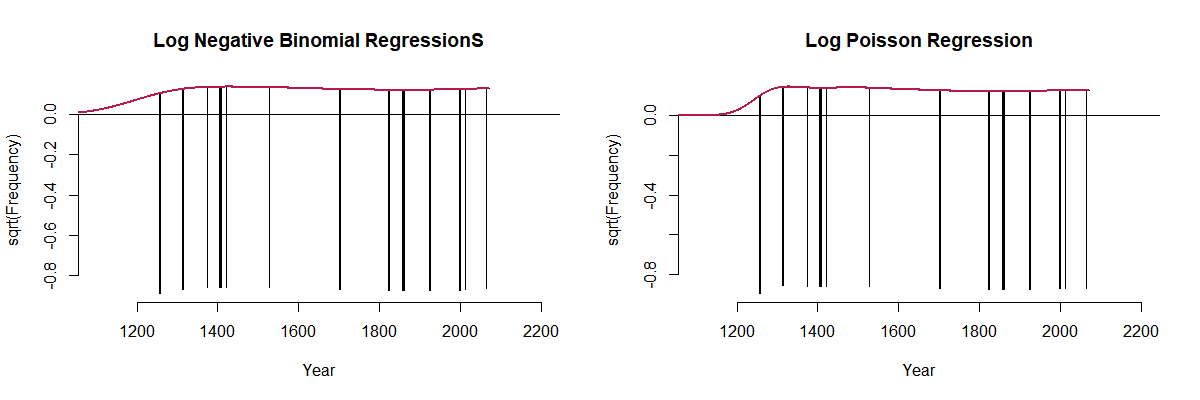
Fig 4. Hang plots of Model (6) (Left) and Model (7) (Right)
Discussion
Compare with the paper’s result
The total non- firearm death results of Chapman, et al is copied as follows. The mean trend of death rate before the law change is equal to exp (0.0212) = 1.021 and its confidence interval has been shown above. The mean trend of death rate after the law change is equal to exp (0.0212 – 0.0348) = 0.986. The 95% confidence interval of this trend is exp (0.0157 – 0.0348) = 0.981 and exp (0.0226 – 0.0348) = 0.992, which is calculated by adding the coefficient of ‘Law’ into the confidence interval of coefficient of (Year - 1996). RT and RL are equal to the rate ratio at the law change and the exponential of the slope difference between the two status which has been shown above in the table.
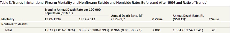
Fig 5. Original results from the paper of Chapman, et al
The association between separate model and combined model
The reason that I didn’t do a separate log Poisson regression before and after the law change is because that they are equivalent with the model (7). Let’s look at model (4) – (6) as an example.
If we substitute the Law value in the model (6) as 0 and 1, which is also the value I generated in the dataset, the model will look like this:
We can see that these two separated models look quite similar with model (4) and model (5). Actually, they are the same. Law = 0 equals to year < 1997, and Law = 1 equals to year >= 1997. If we add the β of Year * Law in model (6) with the β of Year in model (6), we could get the same value of Year’s β in model (5). If we do not add anything to the β of Year in model (6), it equals with the β of Year in model (4). In fact, the β of Year * Law in model (6) describes the differences between the Years’ beta of model (4) and model (5), and we can additionally notice the standard error and p-value of these difference in model (6). That’s why I don’t have to try another separated model for Poisson regression.
Model comparison
From AIC, we can notice that the log negative binomial model fits better than log Poisson regression.
The Log Likelihood of Negative Binomial model is higher than log Poisson, which also means the model (7) fits better.
From the estimating lines (Fig 2.) the two models provided quite same estimating curve, the only difference I noticed is that the end of the blue line (total non-firearm death rate before law change) (in the green circle) in the log Poisson regression is a little bit higher than the log negative binomial regression.
The diagnostic plots of the two models (Fig 3.) are almost the same, the only difference I noticed is in the Q-Q plots. It seems that the error term in log negative binomial regression is better normally distributed than the log Poisson regression.
Limitation
It’s understandable that the rate after the law change is still higher because the rate is just starting to decreasing after the low change by the result of the regressions.
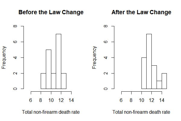
Fig 6. Histogram of total non-firearm death rate in two interested period
However, what we should expect from the law change is that the death rate of firearm could be lower. So, what about the non-firearm deaths? Shall it increase because fewer people will be killed by gunshot? Or shall it be stable because people could still be alive if they avoid the gunshot? Or shall it decrease because people are healthier and healthier? We need a comparison. If we have a global or other comparable total non-firearm death rate, we could know whether the law has actually changed something. If naturally the total non-firearm death rate is decreased after 1996 if some grate medical product has been made, the curve could be same without the law change. After comparing with a counterfactual rate, we could take a deeper insight in to the reason for total non-firearm deaths started to decrease after the law change.
If we do not know the background of the law change, the curve of death rate could be seemed very normal, just a little peak in 1996. Actually, the most obvious change in the raw curve is around 1998 and after 2005. But we do not know whether something important happened at that time. Even there is a cause of raw curve changing happed in the year 1996, we could not distinguish whether it was the law upgrade or other potential mediators and confounders.
The last thing I want to discuss is that the confidence intervals in the model (7) (Log Poisson Regression) is narrower than the model (6) (Log Negative Binomial Regression). However, both the AIC and log-likelihood show that the log negative binomial regression is better. That is because although log Poisson regression is more precise in this case because of its strict distribution assumption, it lost accuracy compare to the negative binomial regression.
Conclusion
This assignment has totally repeated the result of Chapman, et al in the analysis of total non-firearm death rate that the trend of the rate has statistical significantly changed after the year of 1996. From 1979 - 1996, the mean rate of total non-firearm death rate was 10.61 (95%CI, 10.09 - 11.16) per 100,000 person-year (annual trend 1.021, 95%CI: 1.016 - 1.026), whereas from 1997 - 2013, the mean rate of total non-firearm deaths rate was 11.79 (95%CI: 11.21, 12.41) per 100,000 person-year (annual trend 0.986, 95%CI: 0.981, 0.992).
Besides, this assignment compared Log Negative Binomial Regression’s and Log Poisson regression’s performance under this circumstance. The result shows that Log Negative Binomial Regression is better than Log Poisson regression in this case.
Reference:
[1] Chapman, S., Alpers, P., & Jones, M. (2016). Association between gun law reforms and intentional firearm deaths in Australia, 1979-2013. Jama, 316(3), 291-299.