
This is the final assignment of course BIOS 623 at CUNY GSPHHP in Fall 2019
Author: Ruoyan Han
Introduction
Video games, as an emerging merchandise, are usually selling their copies through online stores and physical storage disks. Before a game marked by a price and selling on markets, it should be developed by a developer group and be published by a publisher company. The game prices set by publisher could contain the cost of making the games and advertising fees, which is related to the quality of the games. Steam is the most famous video game digital distribution service developed by Valve Corporation. Most game publishers on the world publish soft copies of games on Steam game store. In the online store, developer, publisher, price, and customers’ reviews are recorded and updated on each game’s web-page.
Overall rating is a count number of all negative reviews (comments) and positive reviews (comments), which in other words is total review numbers (Fig 1). This value should be positively related to sells volume, because on Steam, only players who bought the game can give comments on the web page (one comment per player). The actual selling volume are hidden from the published data I acquired, so that I chose this as dependent variable, which could be considered as a proxy of overall selling volume. In cross-sectional analyses, it is hard to directly analyze the relationship between the game prices with overall ratings. Because the games are not independent with each other, famous publishers and developers could always have some fans love whatever game they made, while small companies may not sell their games well even the quality of the games they made aren’t that worse. Besides, the volume between different publisher are not the same, larger publisher could have more game published in the online stores, which may bias the relationship between price and the game ratings.

In this analysis, I will use different longitudinal models (linear mixed effect models, fixed effect models and generalized estimating equation) to analyze the relationship between game prices and overall ratings in steam online stores among different game publishers. From the results of this analysis, game publishers could see whether the game prices settings is positively or negatively related with overall ratings. And so that they could have a deeper understanding of requirement from player on the view of games prices when they want to publish new games in future.
Method
Data Process
Data Source
Data for this analysis is created by Nik Davis and published on kaggle website [1]. The data collected all available games in U.S. steam online game store in May, 2019. The data is gathered through SteamSpy, a website uses an application programming interface (API) to the Steam software distribution service owned by Valve Corporation to estimate the number of sales of software titles offered on the service created by Sergey Galyonkin [2].
There are several fields in the dataset I acquired and I will use in this analysis:
Publisher ID; Game ID; English (whether the game support English Language), Release Date; Overall Ratings and Price of each game.
Publisher enrolling
To use longitudinal models, multiple published records are needed for each publisher. Besides, small publisher companies who only published two or three games may not show a mature pattern between game price and overall ratings. Therefore, by creating a histogram and looking the distribution of counts of published game, I decided to use publishers who published more than eight games in the analysis.(Fig 2)
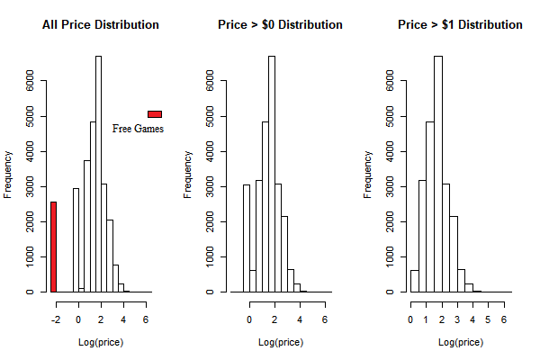
I also excluded free game records in the dataset, although, I reviewed the distribution of published game price (Fig 3) and it dose not show obvious ceiling effect or zero-inflated distribution. It is because that mostly, the commercial mode of free games are not same with the paid games. They usually sell extra components in the game which did not mention in the data. And so that it may bias the relationship between game prices and overall ratings.
Please notice that after removed free games, there could be some publishers have game counts lower than eight.
I also added 0.1 to overall ratings for all games in case that some games’ overall rating is 0, which may not able to do the log transformation. (I would chose to use the log transformation because of the results of descriptive statistics (Fig 4).)
Analyzing Process
Descriptive Statistics
After data cleaning, basic descriptive plots (including game counts distribution, scatter plots of game price, and overall volume) and values (including correlation value, game counts for each publisher) are created and calculated to determine what kind of formats of independent variable and dependent variable to use in the models and cleaning processes.
Cross-sectional Model
To compare the difference between longitudinal models and cross-sectional model, a linear regression is fitted as a comparison. The model is written as following:
$log(\textrm{Overall Ratings}_{i})=\beta_{0}+\beta_{1}*\textrm{Price}_{i}+\xi_{i}$, $i\in\textrm{Publishers}$
The following models are longitudinal models I fitted for the data:
Longitudinal Models (LME)
$log(\textrm{Overall Ratings}_{ij}) = \beta_0 + b_i + \beta_1*(\textrm{Price}_{ij}) + \xi_{ij}$,
$b_i \in N(0, \delta)$, $i\in\textrm{Publishers}$, (LME-1)
Linear Mixed Effect Model - Random Intercept and Slope
$log(\textrm{Overall Ratings}_{ij}) = \beta_0 + b_{i1} + \beta_1*(b_{i2} + \textrm{Price}_{ij}) + \xi_{ij}$,
$b_{i1} \in N(0, \delta_1)$, $b_{i2} \in N(0, \delta_2)$, $i\in\textrm{Publishers}$, $j \in {\textrm{Games of Each Publisher}}$, (LME-2)
Non linear Relationship
$log(\textrm{Overall Ratings}_{ij}) = \beta_0 + b_i + \beta_1(\textrm{Price}_{ij}^2) + \beta_2(\textrm{Price}_{ij}) + \beta_3*(\textrm{Price}_{ij}^{0.5})+ \xi_{ij}$,
$b_i \in N(0, \delta)$, $i\in\textrm{Publishers}$, $j \in {\textrm{Games of Each Publisher}}$, (LME-3)
Effect measurement modifier and confounding effect of whether the game have English version
$log(\textrm{Overall Ratings}_{ij}) = \beta_0 + b_i + \beta_1 (\textrm{Price}_{ij}) + \beta_2 (\textrm{English}_{ij}) + \beta_3 (\textrm{Price}_{ij} \textrm{English}_{ij}) + \xi_{ij}$,
$b_i \in N(0, \delta)$, $i\in\textrm{Publishers}$, $j \in {\textrm{Games of Each Publisher}}$, (LME-4)
Confouder of released date
$log(\textrm{Overall Ratings}_{ij}) = \beta_0 + b_i + \beta_1 (\textrm{Price}_{ij}) + \beta_2 (\textrm{Released Date}_{ij}) + \xi_{ij}$,
$b_i \in N(0, \delta)$, $i\in\textrm{Publishers}$, $j \in {\textrm{Games of Each Publisher}}$, (LME-5)
Estimating line
The estimated value of LME models are calculated and combined with the scatter plots.
Fixed Effect Model (FEM)
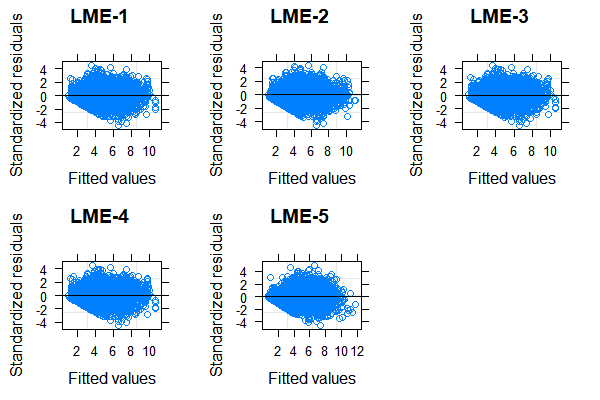
Fixed effect models in this analysis are used to test whether the assumption of LME models (random intercept and random slope) are applicable. Rather than focusing the estimated parameter of ‘price’ in the FEM models, I would pay more attention of the distributions of fixed terms in the models. Distribution of fixed intercepts and slopes are plotted to see whether they are normally distributed. If they are normally distributed, we could use a stronger assumption and use LME the models to fit the data.
Intercept:
$log(\textrm{Overall Ratings}_{ij}) = \alpha_i + \beta_1*(\textrm{Price}_{ij}) + \xi_i$,
$i\in\textrm{Publishers}$, $j \in {\textrm{Games of Each Publisher}}$, (FEM-1)
Slope:
$log(\textrm{Overall Ratings}_{ij}) = \beta_0 + \beta_1 (\textrm{Price}_{ij}) + \beta_2 (\alpha_i * \textrm{Price}_{ij}) + \xi_i$,
$i\in\textrm{Publishers}$, $j \in {\textrm{Games of Each Publisher}}$, (FEM-2)
For the “fixed slopes”, I mean the actually slope of price fitted by this fixed effect model for each publisher.
$\textrm{Fixed Slope} = \beta_1+ \beta_2 * \alpha_i$
I wanted to use the offset() function in the regression of avoid the existence of β2. However, the program did not run well on this. So I still kept the β2. Fortunately, in this case, the existence of β2 does not affect the calculation of ‘fixed slopes’.
Generalized Estimating Equation (GEE)
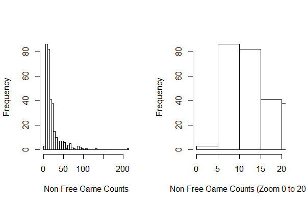
In GEE model, I will use the original overall ratings data because GEE model could handle discreet data. Since the GEE model need same number of records for each publisher. To have a better understanding of correlation matrix, again, I chose the number of game counts in the dataset by the game count distribution (Fig 13). Finally, a subset of GEE model is created by choosing publishers published equal or more than 5 games. And 5 games are randomly chosen into the subset. There are 323 publishers and 1615 games are in the subset.
Before starting to fit the GEE model. Correlation Matrix of 5 games among publishers are calculated and plotted to determine what correlation matrix to use in the GEE model.
Unfortunately, due to technical reason, although I tested the correlation matrix and checked the mean and standard deviation of overall ratings are same or not, I still chose to use Poisson distribution and “exchange” correlation matrix.
$log(\lambda_{ij})= \beta_0 + \beta_1*(\textrm{Price}_{ij})$,
$\textrm{Overall ratings}_{ij} \in Poisson(\lambda_{ij})$,
$i\in\textrm{Publishers}$, $j \in {\textrm{Games of Each Publisher}}$
Tools
Tools I used in this analysis including R software 3.6.1, packages: ggplot2, lattice, gridExtra, nlme, lme4, geepack, stargazer[3], and ggpubr. Microsoft Excel are also used in some calculations.
Results
Data Process
In the raw data, game counts for each publisher are generated and plotted.
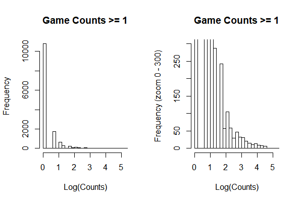
In order to find a proper criteria to remove publishers only publisher one game or published too less game to bias the pattern of prices and overall ratings. From the plot, we can notice that there is a peak around log(counts) = 2, so that I decided to enroll publishers who have published more than exp(2) ≈ 8.
Note: I added 0.1 in the free game prices to generate this plot, otherwise the log price for free games are negative infinity.
From the plot, we can see the distribution of game price is that most game log prices are between 1 and 3. And also there is another peak of game frequency for free games and game prices less than 1 dollar.
The publisher include criteria are created based on the results above. In raw data, their are 14137 game publisher and 27075 published games. Among them, 324 publishers and their 7299 games are selected to be analysis.
In the subset for analysis, distribution of independent variable and dependent variable are plotted as following:
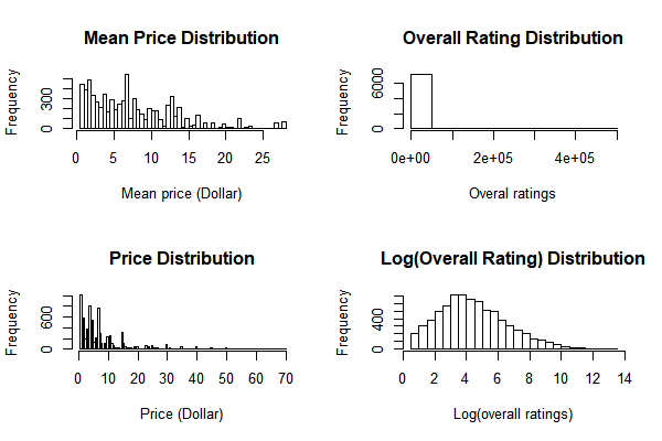
From the plot, we can see that price and mean price do not have an obvious distribution. The original overall ratings have some extremely high value cases, and skewed to the right. The log of overall rating is kind of a unimodal distribution. Therefore, in the longitudinal models, except GEE models (for discrete outcome), I would use the log of overall ratings as the dependent variable.
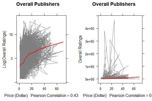
From this plot, we can see that there is a weak correlation between log of overall ratings and price. Especially, over 20 dollars, the smoothed line is almost straight. The correlation for original overall ratings is not obvious.
Analyze Process
As a comparison, a cross-sectional model is fitted.
Table 1. Result of cross-sectional model
| Parameter | Estimation | Standard Error | P-value |
|---|---|---|---|
| Intercept | 3.58 | 0.031 | <0.001 |
| Price | 0.11 | 0.002 | <0.001 |
| R-square | 0.1834 |
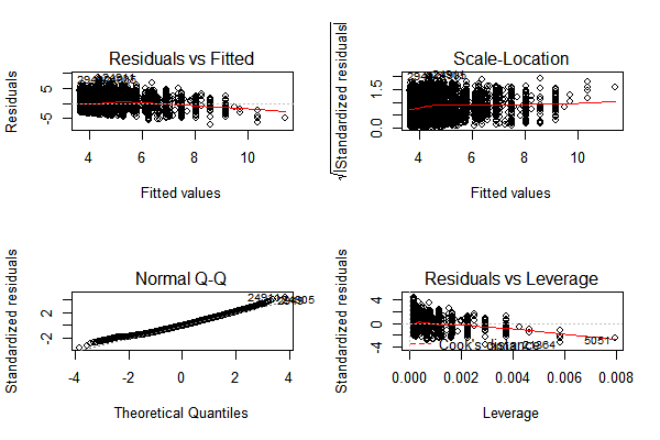
From the results, we can see that the price is positively related to log of overall ratings (p- value < 0.05). However, the R-square is not large, which means the residuals are relatively huge in this model. Other confounders may affect the association.
Table 2. Result of LME Models
| Parameter (Standard Error) | LME-1 | LME-2 | LME-3 | LME-4 | LME-5 |
|---|---|---|---|---|---|
| Price | 0.064*** | 0.058*** | 0.137*** | 0.006 | 0.091*** |
| (Price) | 0.003 | 0.007 | 0.028 | 0.260 | 0.003 |
| Price^0.5 | -0.279** | ||||
| (Price^0.5) | 0.134 | ||||
| Price^2 | -0.001*** | ||||
| (Price^2) | 0.0003 | ||||
| English | 0.351 | ||||
| (English) | 0.250 | ||||
| Price*English | 0.056*** | ||||
| (Price*English) | 0.016 | ||||
| Number of Date to “2019-11-31” | 0.001*** | ||||
| (Number of Date to “2019-11-31”) | 0.00002 | ||||
| Intercept | 3.906*** | 3.932*** | 4.146*** | 3.569*** | 2.720*** |
| (Intercept) | 0.084 | 0.087 | 0.174 | 0.026 | 0.078 |
| —- | —- | —- | —- | —- | —- |
| Random Intercept (Standard Deviation) | 1.43 | 1.43 | 1.43 | 1.44 | 1.18 |
| Random Slope (Standard Deviation) | 0.07 | ||||
| —- | —- | —- | —- | —- | —- |
| Observations | 7299 | 7299 | 7299 | 7299 | 7299 |
| Log Likelihood | -12,942.01 | -12,863.12 | -12,945.80 | -12,927.43 | -12,383.77 |
| Akaike Inf. Crit. | 25,892.02 | 25,738.23 | 25,903.59 | 25,866.86 | 24,777.55 |
| Bayesian Inf. Crit. | 25,919.60 | 25,779.60 | 25,944.96 | 25,908.23 | 24,812.02 |
Note: (*p<0.1); (**p<0.05); (***p<0.01)
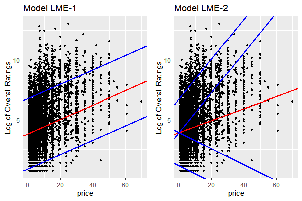
Note: the red lines mean estimated average intercept and slopes. The blues lines are 95% interval of random intercepts and slopes.
Table 3. Fixed Effect Models
| FEM-1 | FEM-2 | |||||
|---|---|---|---|---|---|---|
| Covariates | Estimated Value | Standard Error | P-Value | Estimated Value | Standard Error | P-value |
| price | 0.060 | 0.003 | <0.001 | -0.157 | 0.0356 | 0.6587 |
| Intercept | 3.964 | 0.7923 | <0.001 | |||
| —- | —- | —- | —- | —- | —- | —- |
| Mean of Fixed Term | 3.93 | 0.26 | ||||
| Standard deviation of Fixed Term | 1.49 | 3.26 |
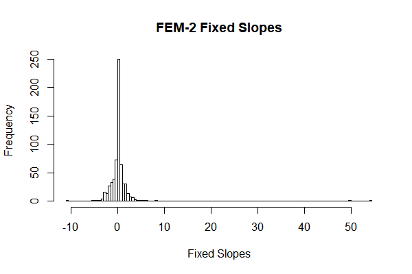
From the results, we can see that both of the fixed intercepts and slopes are quite normally distributed.
Before using GEE model, I generated a subset which contain all the 323 publishers who have more than 5 non-free games in the data and randomly picked 5 games for each publisher. Then randomly picked 100 publishers to fit the GEE model. The reason of why I chose 5 is because the following distribution of free game counts:
To choose what kind of correlated matrix to use in the GEE model, I plotted the correlation of games in five prices. When calculated in the correlation matrix, for each publisher, there could be duplicate prices for publishers. I randomly gave order for same prices.
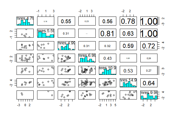
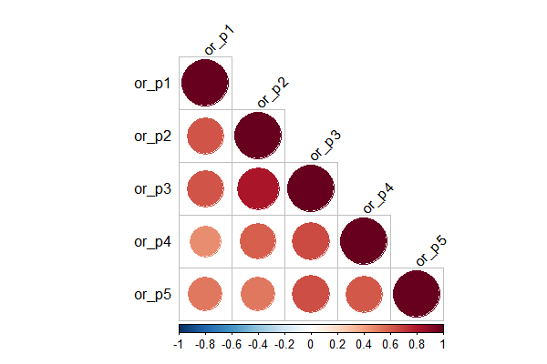
Note: ‘or’ means ‘Overall Ratings’, and ‘p*’ means the rank of five prices
Table 4. Generalized Estimating Equation
| Estimated Value | Standard Error | P-value | |
|---|---|---|---|
| price | 0.0410 | 0.013 | 0.001 |
| Intercept | 6.732 | 0.386 | <0.001 |
Discussion
What are overall ratings indicating? What the models tell the game publishers?
Overall ratings may not be the most import measurement for game publishers, but actually it is the most important variable in the dataset I acquired. Firstly, as mentioned in introduction, the number of overall ratings is positively related to the selling volume. On the other hand, if there are lots of comments, publishers could get many reviews of the game, which could also help publishers and developers editing the game. Therefore, for each game, publishers do expect more comments / higher overall rating. The results of this analysis could help publishers expecting the overall ratings value (the number of total comments) by the setting of game price.
On average, for each publisher, the higher price one game published with, the more comments (higher overall ratings) is expected to acquire. However, this not means that a game with infinity price would have infinity overall rating. From LME models of testing non-linearity (LME-3), and with other covariates (LME4, LME-5) should that there are other factors effecting the relationship between game price and overall ratings. Besides, publishers cannot based on the results to set the game prices unreasonable high. The results can only tell us games with higher price could have higher overall ratings. Actually speaking, to receive higher overall ratings, the publishers should publish games that worth that higher prices.
Which model is the best to describe the relationship between game price and selling volume?
Since there will be many models discussed in this part, I will give my answer at first. In my opinion, the linear effect model with random intercept and random slope describes the relationship in a best way.
Firstly, compare with the cross sectional model, longitudinal models could control for the difference between each publisher, sot hat it could reduce the confounding effect between game prices and overall ratings. The regression coefficient of price in cross-sectional model is higher than the longitudinal models, which means that the proportion of publishers who have more overall ratings is higher in the dataset.
Secondly, for generalized estimating equation, I put too many adjustments in that model. Because GEE model require each publisher have same amount of published games, I removed the publishers who have less than five games in the analyzing dataset and randomly chose five games for publishers who have more than five games. Besides, I should use the “unstructured” correlation model to fit the data. However, it would cost too much times to finish it. And at last, I still use “exchangeable” correlation matrix in the model. And the original count data isn’t a good dependent variable in this case.
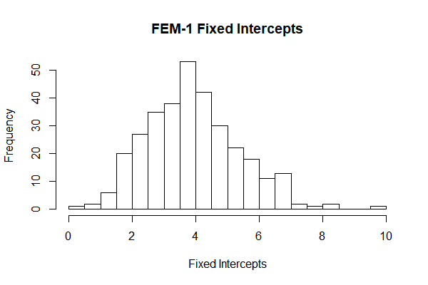
Thirdly, in the fixed effect models, we can see that the fixed intercepts and slopes are quite normally distributed (Fig 9, Fig 10), which means we can make a stronger hypothesis that this intercepts and slopes are normally distributed.
Also from AIC and the Log likelihoods, the LME model with random intercept and random slope was still the best one among models without other covariates.
Whether we should controlling released time in the model?
At first, I do not want to adjust for released date because it is not associated with game price. The common prices setting of video games has not been changed for quite long time. The game with higher quality and made by large game companies (AAA games) would have a price of 59.99 dollars. There are also some lower settings like 49.99 dollars, 29.99 dollars or 23.99 dollars. Actually the setting of game prices is not that clear lower than 49.99 dollars. Although, on the other hand, release time is strongly related to the number of overall ratings, I still did not think released time could be a confounder. However, I noticed that some games would permanently reduced prices after resealed for a long time like about 1 year or 2 years. There are also some games permanently enhanced their prices because the developers made a great update and enhanced the overall game quality. Therefore, I finally included the released time in the analyses. The result shows that, after controlled by released time, the game price is also positively related to the overall ratings.
Limitations of the analysis
In the analysis, there are three spots that I manually decide to remove some records from the dataset. The first one is that I only include publishers who published more than eight games in the analysis. The main reason of doing this is to fit the requirement of longitudinal data that each individual should have several records. Although I did find some evidence from the distribution of published game counts to say patterns from publishers who published more than eight games should be more stable and mature than from new game publishers, it is still lack of scientific supports. The second spot was in the GEE model, because I need reduce the number of records and for each individual publishers, I need same game records. Therefore, I randomly picked 5 games from each publishers.
In longitudinal analysis, both of these problem could have another solution: for example, if there is a publisher only published 2 games and have different game prices and overall ratings, I could estimate overall ratings at other game prices for this publisher by basic algebra. However, there is another problem in this solution: I do not know what price I should estimated by. No one knows if there is another game published by the publisher, what game price would it be set. But all in all, there is data from the original dataset did not include in the model. Therefore, I should set the target population to be game publishers who published more than eight games.
The third spot is that I did not involve free games in the analysis. In reason is that most free games have paid services in the game and it is hard to count it’s price because it’s different by player. However, there could also have few games that actually because of the poor game quality to be set as free games. But I did not include them in the model. Therefore, the result
Another limitation is about the correlation of overall ratings. By introducing longitudinal analysis and setting publishers as individual, the correlation of overall ratings has been counted and fitted in the models. However, Not only there are publishers publish games from different developers, but also there is a few amount of developers who publish their games in different publishers. This means There still could be correlations of overall ratings among different publishers because they published different games from same developers.
There are lots of other variables effect the overall ratings like the types of games, whether the game is published on other platforms and how the publisher advertising the game. Further analysis could concern more covariates to make the mechanism of how prices effects overall ratings clearer.
Conclusion
This analysis shows that on average, game price is positively related to the overall ratings. For one dollar increased on the game price for one publisher among publishers who published more than eight games, there is about 0.06 promotion in log overall rating of the game. This analysis also proved that this positively relationship is not linear. And games’ overall rating could also be effect by other variables like whether the game have English version or released date.
Reference
[1] Nik Davis, (2019) Steam Store Games (Clean dataset)
Combined data of 27,000 games scraped from Steam and SteamSpy APIs, https://www.kaggle.com/nikdavis/steam-store-games
[2]Wikipedia contributors. (2019, December 3). Steam Spy. In Wikipedia, The Free Encyclopedia. Retrieved 21:08, December 12, 2019, from https://en.wikipedia.org/w/index.php?title=Steam_Spy&oldid=929122689
[3] Hlavac, Marek (2018). stargazer: Well-Formatted Regression and Summary Statistics Tables. R package version 5.2.2. https://CRAN.R-project.org/package=stargazer