
Author: Ruoyan Han
Code and data for this case is available at:
https://github.com/Ry2an/case_code/tree/master/bios623as3
Introduction:
This practicing case is going to repeat partial work of Wondwossen, et al’s paper1.Their paper is focusing on whether the mortality is different of tuberculosis patients who also have HIV when receiving cART treatment at different time points (first week, fourth week and eighth week). This case is mainly repeating Figure 2 and Table 2 of the paper, which included survival analysis by using Kaplan Meier function and Proportional Hazard approach with several corvariates. In addition, residuals of different models are shown and interpreted in this document.
Methods
Data Source:
The dataset used in this paper is included in the supplement of Wondwossen, et al’s paper.
Software:
R software 3.6.1
Package: survival, survminer
Analysis Process:
To repeat the Figure 2 of the original paper, survfit() and survdiff() from R package ‘survival’ are used to calculate. The group setting of Kaplan Meier approach is by three different time of receiving cART. The plot of survival curve and risk table is generated by ggsurvplot() function of package ‘survminer’.
A log rank test is implemented by survdiff() function under R package ‘survival’ to tell whether the survival curve of treatments happened in the week 1, week 4 and week 8 are different with each other.
Univariate Analysis:
Four models are implemented separately by only enrolling treatment, whether CD4 cell count is less than 50 per microliter, whether albumin is less than 3 grams per deciliter and Body Mass Index in the models. This analysis uses coxph() function under R package ‘survival’. The models are listed as following (1 - 4):
Multivariable Analysis:
One model is fitted by enrolling all covariates mentioned in the univariate analysis. The model is shown as following (5):
Martingale, Deviance and Scaled Schoenfeld Residual are drawn in R. Smoothed lines are drawn by the smooth.spline() function in R on each graphs. Additionally, Schoenfeld Residuals are also shown by cox.zph() function under ‘survival’ package in R.
Results
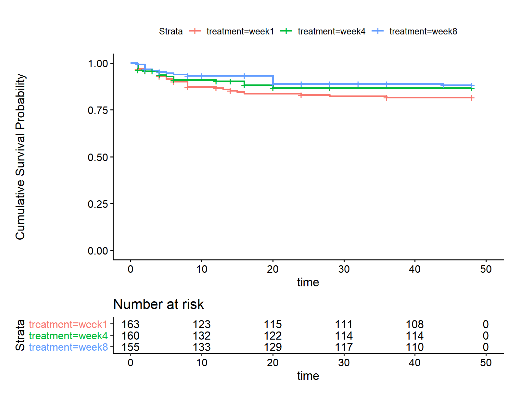
Fig 1. Survival Curve and Risk Table of Kaplan Meier Approach
From the plot, we can see that the survival curve of people who received cART treatment in 8th week remains staying on the top of other two curves in the study period. Curves of ‘week 1’ and ‘week 4’ treatments have some crosses before the first 10 weeks. Then the curves of ‘week 1’ keeps staying at the bottom of the three curves.
Table 1. Result of Log - Rank Test
| Treatment | N | Observed | Expected | (O-E)^2/E | (O-E)^2/V |
|---|---|---|---|---|---|
| week1 | 163 | 27.00 | 20.90 | 1.78 | 2.68 |
| week4 | 160 | 20.00 | 21.56 | 0.11 | 0.17 |
| week8 | 155 | 17.00 | 21.54 | 0.96 | 1.47 |
| Chi-Square Value | 2.89 | Degree of Freedom | 2.00 | p-value | 0.24 |
Table 2. Estimated Values of Univariable Models (1 - 4) and the Multivariable Models (5)
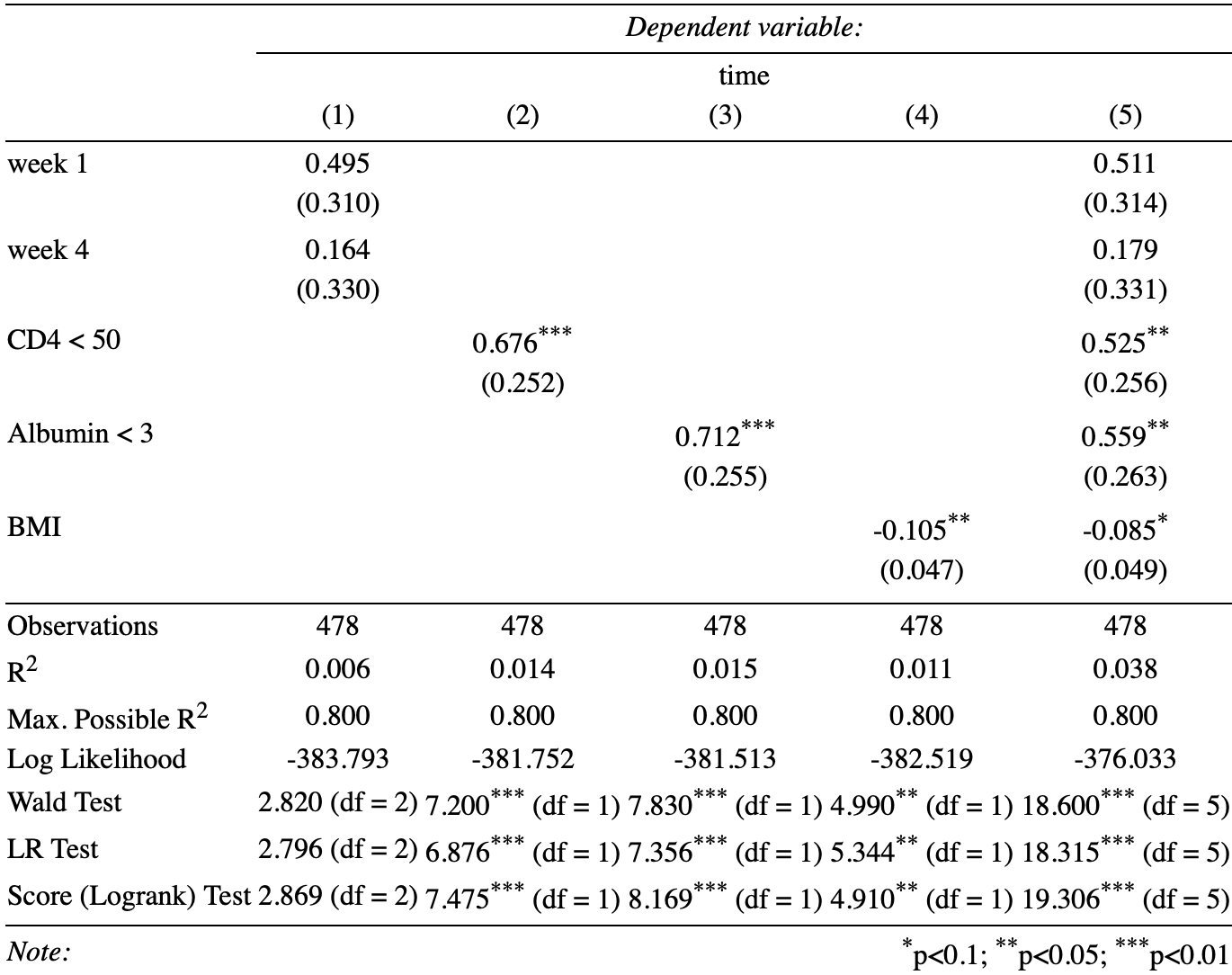
The results of univariate analysis show that the hazard ratio of ‘week 8’ group compared by ‘week 1’ group and ‘week 4’ group are both not statistically significant by 1 (both parameters not statistically significant by 0). However, parameter of CD4, Albumin conditions and BMI are statistically significant than 0 at 0.05 critical criteria.
In the multivariable analysis, the conditions of the p-values for covariates are roughly the same with the univariate analysis. Both parameter of ‘week 1’ and ‘week 4’ treatments are not statistically significant by 0. The parameter of CD4, Albumin and conditions are statistically significant than 0 at 0.05 critical criteria. The only difference happened in the parameter ‘BMI’. It is significant at 0.1 critical criteria but not significant at 0.05 critical criteria.
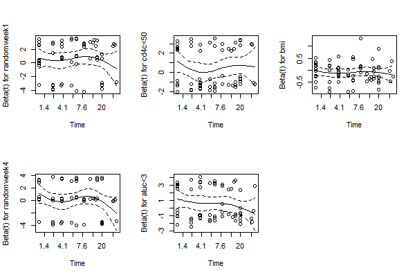
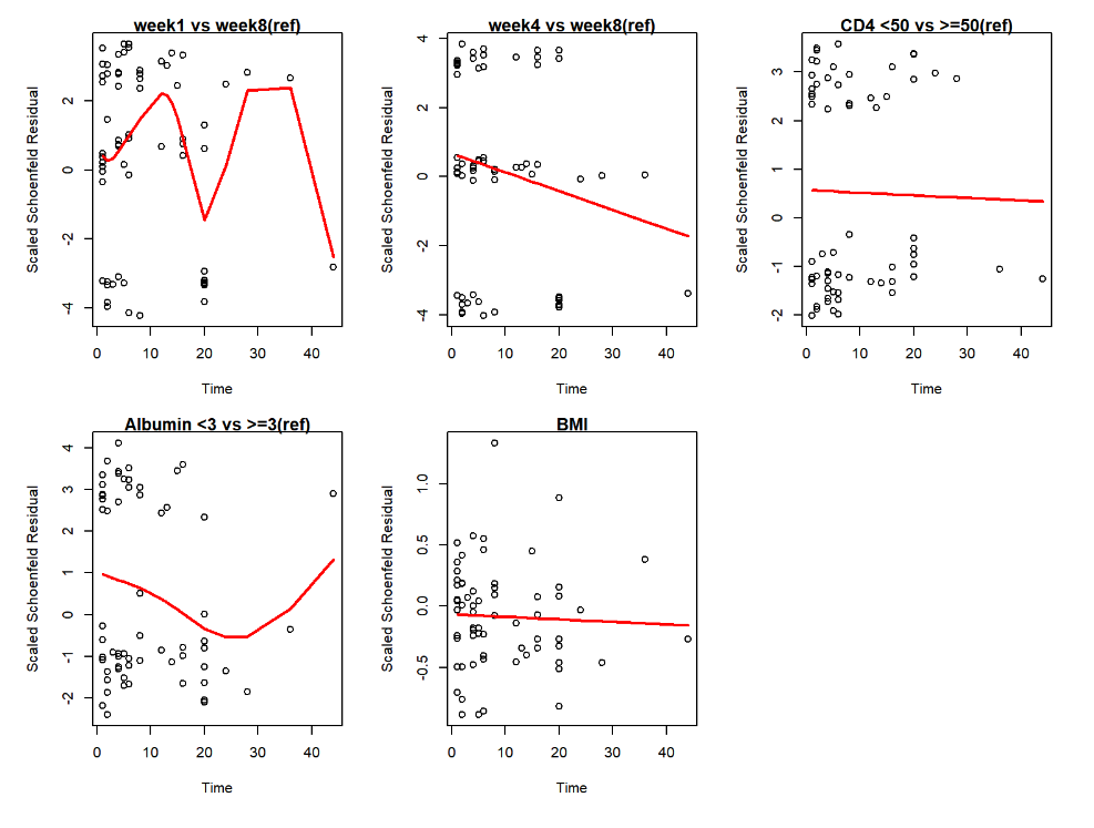
Fig 2. Scaled Schenfeld Residual for Each Covariates in Multivariable Analysis
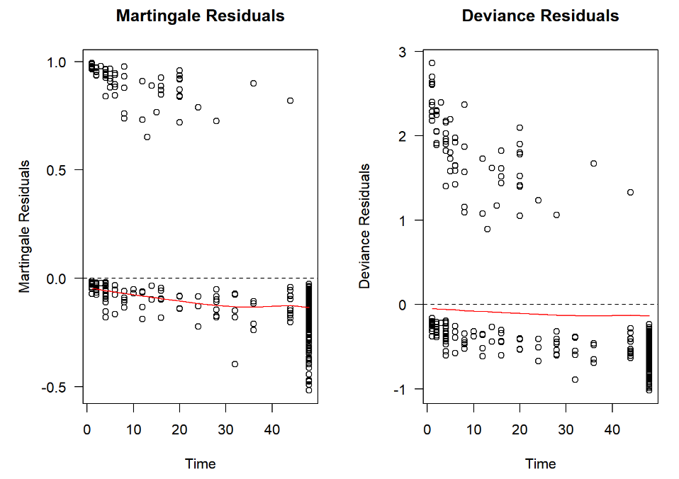
Fig 3. Matingale Residuals and Deviance Residuals
All of the residuals lying close to ‘0’. For Schenfeld residuals, we can the confidence intervals are always contain 0 for each covariates. This indicates that the multivariable model has a good fit so that the error term could stay in the distribution assumed by the model.
Discussion
There are several discrepancy between my results with the original paper. In the univariate analysis multivariable analysis, the regression coefficient of ‘CD4’ and ‘Albumin’ are not same with the paper. Coefficient of ‘Week 1’ are not same in the multivariable analysis. I think the reason is because of the data from the supplement of the paper. Although I analyzed with people who lost follow up before the treatment by considering the intention to treat approach, which was the same as the authors did in their paper, we can see that there are discrepancy between the number of people who died or quit before the treatment. In the paper, the number of three groups (‘week1’, ‘week4’ and ‘week8’) who received the treatment is 149, 147 and 135, while from the data they are 150, 146, and 137. This could lead the survival probability of three treatments different with the original paper at least when first event happens. Besides, In this assignment, I didn’t include ‘Hepatotoxicity requiring interruption of TB therapy’ as a covariate in the model, which could also lead different results.
Table 3. Comparation Between Hazard Ratio in Previous Model and in the Original Paper
| Covariates | Univariate Model | Multivariable Model | ||||||
|---|---|---|---|---|---|---|---|---|
| Hazard Ratio | HR From Paper | p-value | p-value from paper | Hazard Ratio | HR From Paper | p-value | p-value from paper | |
| Week 1 | 1.64 | 1.6 | 0.110 | 0.1 | 1.67 | 1.5 | 0.104 | 0.2 |
| Week 4 | 1.18 | 1.2 | 0.620 | 0.6 | 1.20 | 1.2 | 0.588 | 0.6 |
| CD4 cell < 50 | 1.97 | 3.3 | 0.007 | 0.001 | 1.69 | 2.7 | 0.041 | 0.001 |
| Albumin < 3 | 2.04 | 2.8 | 0.005 | 0.001 | 1.75 | 2.3 | 0.033 | 0.02 |
| BMI | 0.90 | 0.9 | 0.025 | 0.0 | 0.92 | 0.9 | 0.079 | 0.04 |
Although the parameters of different treatments are not significant in the model, we can still see a trend among three treatments:
Hazard Ratio: week 1 : week 8 = 1.7; week 4 : week 8 = 1.2; week 8 : week 8 = 1. It is obvious that by controlling with other covariates, the later the patient receive the treatments, the higher of the survival probability could be. But it’s just not statistically significant.
In my opinion, there could be two solutions to figure out whether there is a trend between treatment time point and survival probability. The first one is to increase the sample size. I will use the parameter of ‘week 1’ in the multivariable analysis as an example. The standard error of this parameter is 0.314, which means only when the regression coefficient is larger than about 0.314 * 1.96 = 0.615 (negatively calculate is the same mechanism), it could be statistically significant at 0.05 critical criteria. That means the hazard ratio compare ‘week 8’ with ‘week 1’ should be larger than exp(0.615) = 1.85. However, as far as I am concerned, 1.5, or 1.2 are still meaningful results for the context. It’s just the study do not have enough power to prove it is statistically significant. In another words, if the standard error of ‘week 1’ could reduced to about 0.511 / 1.96 = 0.261, the result could be statistically significant at 0.05 critical criteria. We know that in the ‘week 1’ group, there are 163 participants, which means the variance of the regression coefficient in target population could be estimated as 0.314 * (163)^0.5 = 4.01. If we want the standard error (the variance of the sample mean of the regression coefficient from target population) to be less than 0.261, the sample size of the treatment group should be more than (4.01 / 0.261)^2 = 236. It is not a huge number, if the study could also increase the number of participants in ‘week 8’, the number could be lesser.
Another solution is to find another approach by assuming the outcome variable do have an order, with stronger assumption, the parameters could be farther to null hypothesis.
Conclusion:
From current results, we cannot deny the hypothesis that treatments in three different times could lead same survival curve, which means the hazard ratio of ‘week 1’ and ‘week 4’ compare to ‘week 8’ are same with 1. However, from the result, we could notice that other covariates like baseline CD4, Albumin and BMI status could be more related to different cumulative survival probability by time in the target population.
Reference:
[1] Amogne, W., Aderaye, G., Habtewold, A., Yimer, G., Makonnen, E., Worku, A., … & Lindquist, L. (2015). Efficacy and safety of antiretroviral therapy initiated one week after tuberculosis therapy in patients with CD4 counts< 200 cells/μL: TB-HAART Study, a randomized clinical trial. PLoS One, 10(5), e0122587.