
This is a note of learning SIR model, which means Suscepted - Infected - Recovered Model.
Background Kowledge of the Model
Assume we have a group of people. This group of people is very stable, there is no dying, no birth among them. They are living in a isolated area and there is no move in and move out. And thus, the total count of this group of people is stable.
Unfortunately, someday, a small number of people among them got an infectious disease. Appreciated to our human inmmunity system, once people recoved from the disease, B cells can remember it and protect its host not get infected again.
Therefore, assumming all people in this group is susceptable for this disease at the begining, this group of people could have three components: suscepted, infected and recovered. In this special stable group, we can know that all of them would go through the suscept, infect and recover processes and finally this disease can no longer cause anything in this group of people.
Formulas of the Model
However, describing the trend of the three componnets, is not as easy as the ‘swimming pool questions’ we learned in primary schools. But we can still have a little galnce review of it. Assume there are three swimming pools in your backyard called “Suscept”, “Infect” and “Recover”. Waters are slowly flowing from “S”, through “I” and finally moving to “R”. We can know that the relationship between remain volume in three pools are:

However, the biggest problem of these equation is that the speed among the pools are not stable!
If we know something about infectious diseases, we can know that:
The more infected people in that group, the faster the people “flowing from S to I”.
The more infected people there is, if the chance of recovering for each patient is same, the more people “flowing from I to R.”
And in fact, during the process that everyone tranforming from S to R, the number of I is actually changing all the time.
A good thing is that we can define the “speed of transforming per unit time” in formulas above based on these features.
We can set the speed of S to I as $\beta_1*\textrm{S}*\textrm{I}$, and the speed of I to R as $\beta_2*\textrm{I}$. Thus, the formulas are chaged as following:
Shiny Program
I also created a R shiny app to simulate the trends, please use the following code in your R studio:
1 | library(shiny) |
To install shiny package, you may want to use:
1 | install.packages("shiny") |
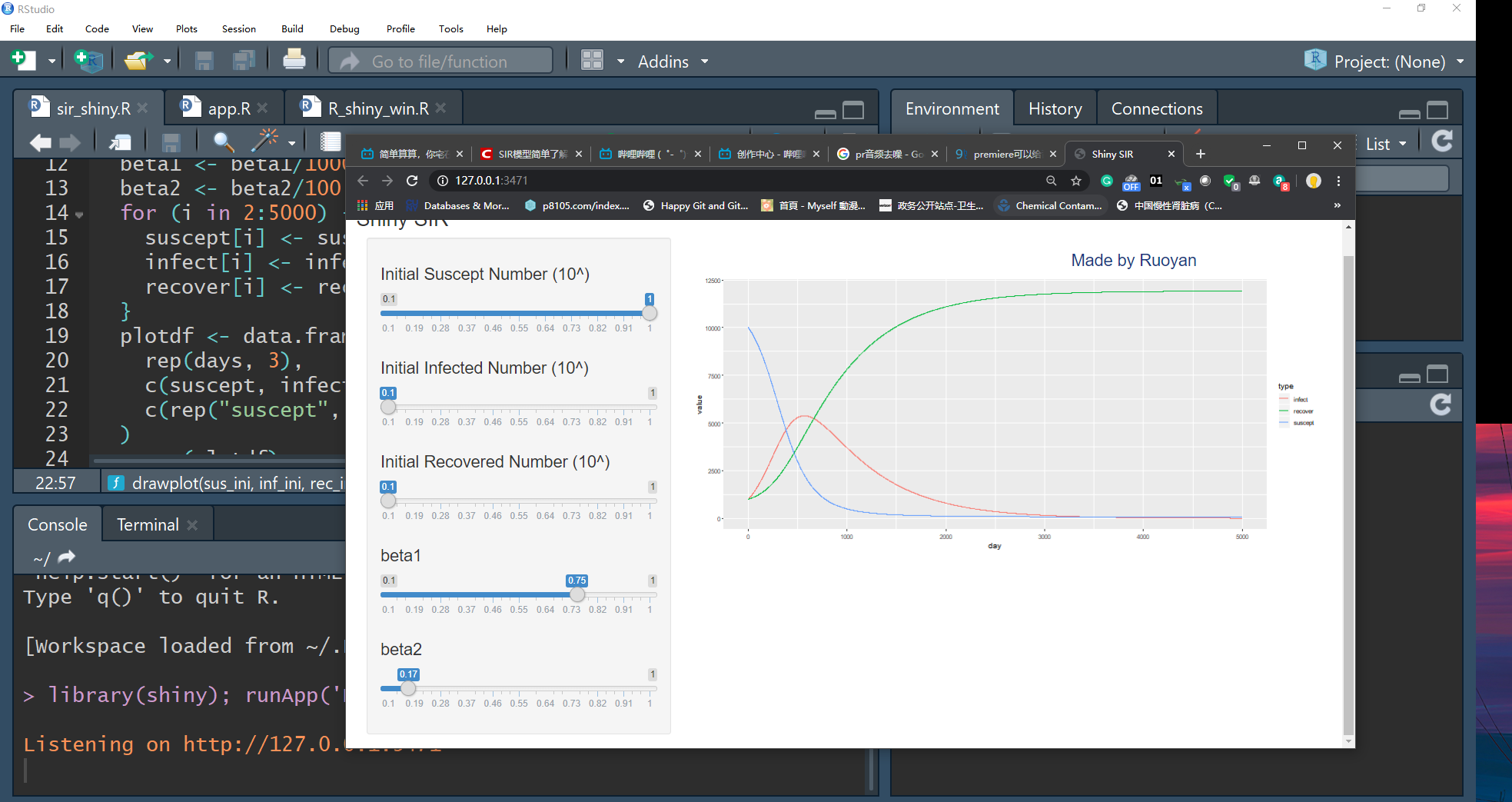
Here is a snapshot of the Shiny App.
Video tutorial
I created a video to show how the model works and how to draw the curves through R and ggplot2. The video is published on bilibili video site. I apologize that there is no English subtitle in that video, but the code should be clear to see.
Thank you for reading my article!